使用离线批推理进行模型验证#

本教程执行一个批推理工作负载，该工作负载连接了以下异构工作负载：

从云存储进行分布式读取
分布式预处理
并行批推理
分布式汇总指标聚合

请注意，本教程从分布式训练 XGBoost 模型教程中获取预训练的模型伪影。

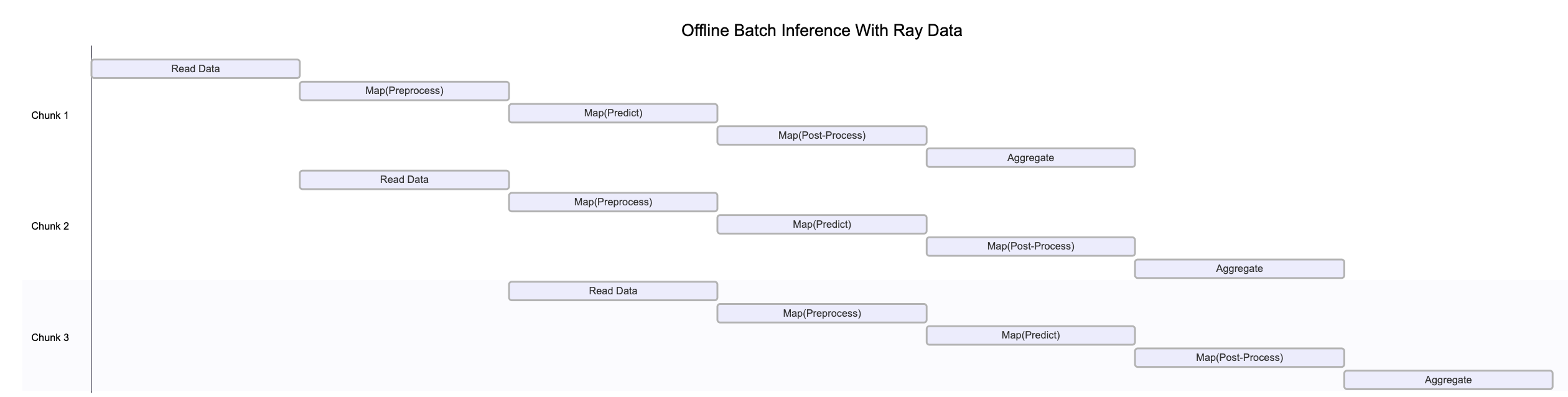
https://raw.githubusercontent.com/anyscale/e2e-xgboost/refs/heads/main/images/batch_inference.png

上图说明了 Ray Data 如何在管道的各个阶段同时处理不同数据块。这种并行执行最大化了资源利用率和吞吐量。

请注意，此图为简化示意图，原因如下：

背压机制可能会限制上游算子，以防止下游阶段过载。
数据在管道中移动时，动态重分区经常发生，改变块的数量和大小。
随着集群自动伸缩，可用资源会发生变化。
系统故障可能会中断图中显示的清晰顺序流程。

Ray Data 流式执行

❌ **传统批处理执行**，非流式处理，如不带流水线的 Spark 和 SageMaker Batch Transform

将整个数据集读入内存或持久化中间格式。
然后才开始应用转换，如 .map、.filter 等。
内存压力更高，启动延迟更高。

✅ Ray Data 的**流式执行**

加载数据块（“blocks”）后立即开始处理，无需等待整个数据集加载完成。
降低内存占用，避免出现内存不足错误，并加快首次输出速度。
通过减少空闲时间来提高资源利用率。
实现低延迟的在线推理管道。

https://raw.githubusercontent.com/anyscale/e2e-xgboost/refs/heads/main/images/streaming.gif

注意：Ray Data 并不是一个实时流处理引擎，如 Flink 或 Kafka Streams。相反，它是一种具有流式执行能力的批处理引擎，这对于迭代式机器学习工作负载、ETL 管道以及训练或推理前的预处理特别有用。与 Spark 和 SageMaker Batch Transform 等解决方案相比，Ray 通常能实现 **2-17 倍的吞吐量提升**。

%load_ext autoreload
%autoreload all

# Enable importing from dist_xgboost package.
import os
import sys

sys.path.append(os.path.abspath(".."))

# Enable Ray Train v2.
os.environ["RAY_TRAIN_V2_ENABLED"] = "1"
# Now it's safe to import from ray.train.

import ray
import dist_xgboost

# Initialize Ray with the dist_xgboost package.
ray.init(runtime_env={"py_modules": [dist_xgboost]})

# Configure Ray Data logging.
ray.data.DataContext.get_current().enable_progress_bars = False
ray.data.DataContext.get_current().print_on_execution_start = False

使用 Ray Data 验证模型#

上一教程《使用 XGBoost 进行分布式训练》训练了一个 XGBoost 模型并将其存储在 MLflow 的伪影存储中。在此步骤中，使用该模型对保留的测试集进行预测。

数据摄取#

使用与之前相同的过程加载测试数据集。

from ray.data import Dataset


def prepare_data() -> tuple[Dataset, Dataset, Dataset]:
    """Load and split the dataset into train, validation, and test sets."""
    dataset = ray.data.read_csv("s3://anonymous@air-example-data/breast_cancer.csv")
    seed = 42
    train_dataset, rest = dataset.train_test_split(test_size=0.3, shuffle=True, seed=seed)
    # 15% for validation, 15% for testing.
    valid_dataset, test_dataset = rest.train_test_split(test_size=0.5, shuffle=True, seed=seed)
    return train_dataset, valid_dataset, test_dataset


_, _, test_dataset = prepare_data()
# Use `take()` to trigger execution because Ray Data uses lazy evaluation mode.
test_dataset.take(1)

2025-04-16 21:14:42,328	INFO worker.py:1660 -- Connecting to existing Ray cluster at address: 10.0.23.200:6379...
2025-04-16 21:14:42,338	INFO worker.py:1843 -- Connected to Ray cluster. View the dashboard at https://session-1kebpylz8tcjd34p4sv2h1f9tg.i.anyscaleuserdata.com 
2025-04-16 21:14:42,343	INFO packaging.py:575 -- Creating a file package for local module '/home/ray/default/e2e-xgboost/dist_xgboost'.
2025-04-16 21:14:42,346	INFO packaging.py:367 -- Pushing file package 'gcs://_ray_pkg_fbb1935a37eb6438.zip' (0.02MiB) to Ray cluster...
2025-04-16 21:14:42,347	INFO packaging.py:380 -- Successfully pushed file package 'gcs://_ray_pkg_fbb1935a37eb6438.zip'.
2025-04-16 21:14:42,347	INFO packaging.py:367 -- Pushing file package 'gcs://_ray_pkg_534f9f38a44d4c15f21856eec72c3c338db77a6b.zip' (0.08MiB) to Ray cluster...
2025-04-16 21:14:42,348	INFO packaging.py:380 -- Successfully pushed file package 'gcs://_ray_pkg_534f9f38a44d4c15f21856eec72c3c338db77a6b.zip'.
2025-04-16 21:14:44,609	INFO dataset.py:2809 -- Tip: Use `take_batch()` instead of `take() / show()` to return records in pandas or numpy batch format.

[{'mean radius': 15.7,
  'mean texture': 20.31,
  'mean perimeter': 101.2,
  'mean area': 766.6,
  'mean smoothness': 0.09597,
  'mean compactness': 0.08799,
  'mean concavity': 0.06593,
  'mean concave points': 0.05189,
  'mean symmetry': 0.1618,
  'mean fractal dimension': 0.05549,
  'radius error': 0.3699,
  'texture error': 1.15,
  'perimeter error': 2.406,
  'area error': 40.98,
  'smoothness error': 0.004626,
  'compactness error': 0.02263,
  'concavity error': 0.01954,
  'concave points error': 0.009767,
  'symmetry error': 0.01547,
  'fractal dimension error': 0.00243,
  'worst radius': 20.11,
  'worst texture': 32.82,
  'worst perimeter': 129.3,
  'worst area': 1269.0,
  'worst smoothness': 0.1414,
  'worst compactness': 0.3547,
  'worst concavity': 0.2902,
  'worst concave points': 0.1541,
  'worst symmetry': 0.3437,
  'worst fractal dimension': 0.08631,
  'target': 0}]

💡 Ray Data 最佳实践

开发期间使用 materialize()：materialize() 方法会在 Ray 的共享内存对象存储中执行并存储数据集。这种行为会创建一个检查点，以便将来的操作可以从此点开始，而无需从头开始重新运行所有操作。
选择合适的混洗策略：Ray Data 提供了各种混洗策略，包括局部混洗和每个 epoch 的混洗。您需要混洗此数据集，因为原始数据按类别对项目进行分组。

接下来，以与训练期间相同的方式转换输入数据。从伪影注册表中获取预处理器。

import pickle

from dist_xgboost.constants import preprocessor_fname
from dist_xgboost.data import get_best_model_from_registry

best_run, best_artifacts_dir = get_best_model_from_registry()

with open(os.path.join(best_artifacts_dir, preprocessor_fname), "rb") as f:
    preprocessor = pickle.load(f)

现在，在 Ray Data 管道中定义转换步骤。不要使用 .map() 单独处理每个项目，而是使用 Ray Data 的 map_batches 方法一次处理整个批次，这样效率更高。

def transform_with_preprocessor(batch_df, preprocessor):
    # The preprocessor doesn't include the `target` column,
    # so remove it temporarily, then add it back.
    target = batch_df.pop("target")
    transformed_features = preprocessor.transform_batch(batch_df)
    transformed_features["target"] = target
    return transformed_features


# Apply the transformation to each batch.
test_dataset = test_dataset.map_batches(
    transform_with_preprocessor,
    fn_kwargs={"preprocessor": preprocessor},
    batch_format="pandas",
    batch_size=1000,
)

test_dataset.show(1)

{'mean radius': 0.4202879281965173, 'mean texture': 0.2278148207774012, 'mean perimeter': 0.35489846800755104, 'mean area': 0.29117590184541364, 'mean smoothness': -0.039721410464208406, 'mean compactness': -0.30321758777095337, 'mean concavity': -0.2973304995033593, 'mean concave points': 0.05629912285695481, 'mean symmetry': -0.6923528276633714, 'mean fractal dimension': -1.0159489469979848, 'radius error': -0.1244372811541358, 'texture error': -0.1073358496664629, 'perimeter error': -0.2253381140213174, 'area error': 0.001804996358367429, 'smoothness error': -0.8087740189276656, 'compactness error': -0.1437977993323648, 'concavity error': -0.3926326901399853, 'concave points error': -0.34157926393517024, 'symmetry error': -0.5862955941365042, 'fractal dimension error': -0.496152478599194, 'worst radius': 0.7695260874215265, 'worst texture': 1.1287525414418031, 'worst perimeter': 0.6310282171135395, 'worst area': 0.6506421499178707, 'worst smoothness': 0.39052158034274154, 'worst compactness': 0.6735246675401986, 'worst concavity': 0.06668871795848759, 'worst concave points': 0.5859784499947507, 'worst symmetry': 0.8525444557664399, 'worst fractal dimension': 0.14066370266791928, 'target': 0}

加载已训练模型#

现在您已经定义了预处理管道，可以运行批推理了。从伪影注册表中加载模型。

from ray.train import Checkpoint
from ray.train.xgboost import RayTrainReportCallback

checkpoint = Checkpoint.from_directory(best_artifacts_dir)
model = RayTrainReportCallback.get_model(checkpoint)

运行批推理#

接下来，运行推理步骤。为了避免为每个批次重复加载模型，请定义一个可重用类，该类可以使用相同的 XGBoost 模型处理不同的批次。

import pandas as pd
import xgboost

from dist_xgboost.data import load_model_and_preprocessor


class Validator:
    def __init__(self):
        _, self.model = load_model_and_preprocessor()

    def __call__(self, batch: pd.DataFrame) -> pd.DataFrame:
        # Remove the target column for inference.
        target = batch.pop("target")
        dmatrix = xgboost.DMatrix(batch)
        predictions = self.model.predict(dmatrix)

        results = pd.DataFrame({"prediction": predictions, "target": target})
        return results

现在，通过分批处理数据来并行化模型的推理。

test_predictions = test_dataset.map_batches(
    Validator,
    concurrency=4,  # Number of model replicas.
    batch_format="pandas",
)

test_predictions.show(1)

2025-04-16 21:14:56,496	WARNING actor_pool_map_operator.py:287 -- To ensure full parallelization across an actor pool of size 4, the Dataset should consist of at least 4 distinct blocks. Consider increasing the parallelism when creating the Dataset.

{'prediction': 0.031001044437289238, 'target': 0}

计算评估指标#

现在您有了预测结果，可以评估模型的准确率、精确率、召回率和 F1 分数。计算测试子集上的真阳性、真阴性、假阳性和假阴性数量。

from sklearn.metrics import confusion_matrix


def confusion_matrix_batch(batch, threshold=0.5):
    # Apply a threshold to get binary predictions.
    batch["prediction"] = (batch["prediction"] > threshold).astype(int)

    result = {}
    cm = confusion_matrix(batch["target"], batch["prediction"], labels=[0, 1])
    result["TN"] = cm[0, 0]
    result["FP"] = cm[0, 1]
    result["FN"] = cm[1, 0]
    result["TP"] = cm[1, 1]
    return pd.DataFrame(result, index=[0])


test_results = test_predictions.map_batches(confusion_matrix_batch, batch_format="pandas", batch_size=1000)

最后，将所有批次的混淆矩阵结果聚合起来，得到全局计数。此步骤将具体化数据集并执行所有先前声明的惰性转换。

# Sum all confusion matrix values across batches.
cm_sums = test_results.sum(["TN", "FP", "FN", "TP"])

# Extract confusion matrix components.
tn = cm_sums["sum(TN)"]
fp = cm_sums["sum(FP)"]
fn = cm_sums["sum(FN)"]
tp = cm_sums["sum(TP)"]

# Calculate metrics.
accuracy = (tp + tn) / (tp + tn + fp + fn)
precision = tp / (tp + fp) if (tp + fp) > 0 else 0
recall = tp / (tp + fn) if (tp + fn) > 0 else 0
f1 = 2 * precision * recall / (precision + recall) if (precision + recall) > 0 else 0

metrics = {"precision": precision, "recall": recall, "f1": f1, "accuracy": accuracy}

2025-04-16 21:15:01,144	WARNING actor_pool_map_operator.py:287 -- To ensure full parallelization across an actor pool of size 4, the Dataset should consist of at least 4 distinct blocks. Consider increasing the parallelism when creating the Dataset.

print("Validation results:")
for key, value in metrics.items():
    print(f"{key}: {value:.4f}")

Validation results:
precision: 0.9464
recall: 0.9815
f1: 0.9636
accuracy: 0.9535

以下是预期输出：

Validation results:
precision: 0.9574
recall: 1.0000
f1: 0.9783
accuracy: 0.9767

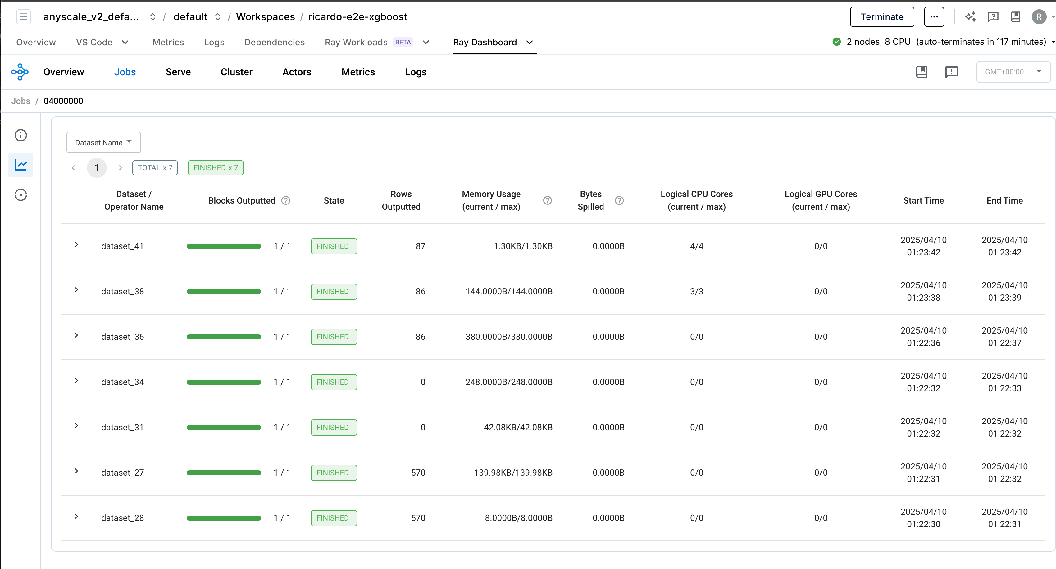
可观察性#

Ray Data 提供了内置的可观测性功能，可帮助您监控和调试数据处理管道。

https://raw.githubusercontent.com/anyscale/e2e-xgboost/refs/heads/main/images/ray_data_observability.png

生产部署#

您可以将培训工作负载包装成生产级的 Anyscale 作业。请参阅 API 参考。

# Production batch job.
anyscale job submit --name=validate-xboost-breast-cancer-model \
  --containerfile="${WORKING_DIR}/containerfile" \
  --working-dir="${WORKING_DIR}" \
  --exclude="" \
  --max-retries=0 \
  -- python dist_xgboost/infer.py

请注意，为了使此命令成功，请先配置 MLflow，使其将伪影存储在跨集群可读的存储中。Anyscale 提供各种开箱即用的存储选项，例如默认存储桶，以及集群、用户和云级别共享的自动挂载的网络存储。您也可以设置自己的网络挂载或存储桶。

总结#

在本教程中，您：

使用从云存储进行的分布式读取加载了测试数据集。
以流式方式转换了数据集，使用了与训练期间相同的预处理器。
进行了一个验证管道，以：
- 使用多个模型副本对测试数据进行预测。
- 为每个批次计算混淆矩阵的组成部分。
- 跨所有批次聚合结果。
计算了关键性能指标，如精确率、召回率、F1 分数和准确率。

使用 Ray Data 的分布式处理能力，相同的代码可以高效地在 TB 级数据集上运行，而无需修改。

下一教程将展示如何使用 Ray Serve 为在线推理服务此 XGBoost 模型。