分析 Tune 实验结果

本指南将介绍在使用 tuner.fit() 运行 Tune 实验后，您可能想要执行的一些常见分析工作流程。

1. 从目录加载 Tune 实验结果

2. 基础实验级分析：快速了解各试验的表现

3. 基础试验级分析：访问单个试验的超参数配置和最后报告的指标

4. 绘制试验报告指标的完整历史记录

5. 访问保存的检查点（假设您已启用检查点功能）并加载到模型中进行测试推理

result_grid: ResultGrid = tuner.fit()
best_result: Result = result_grid.get_best_result()

tuner.fit() 的输出是 ResultGrid，它是 Result 对象的集合。有关可用属性的更多详细信息，请参阅 ResultGrid 和 Result 的链接文档参考。

让我们从使用 MNIST PyTorch 示例执行超参数搜索开始。训练函数定义在这里，我们将其传递给 Tuner 以并行运行试验。

import os

from ray import tune
from ray.tune import ResultGrid
from ray.tune.examples.mnist_pytorch import train_mnist

storage_path = "/tmp/ray_results"
exp_name = "tune_analyzing_results"
tuner = tune.Tuner(
    train_mnist,
    param_space={
        "lr": tune.loguniform(0.001, 0.1),
        "momentum": tune.grid_search([0.8, 0.9, 0.99]),
        "should_checkpoint": True,
    },
    run_config=tune.RunConfig(
        name=exp_name,
        stop={"training_iteration": 100},
        checkpoint_config=tune.CheckpointConfig(
            checkpoint_score_attribute="mean_accuracy",
            num_to_keep=5,
        ),
        storage_path=storage_path,
    ),
    tune_config=tune.TuneConfig(mode="max", metric="mean_accuracy", num_samples=3),
)
result_grid: ResultGrid = tuner.fit()

从目录加载实验结果

虽然由于刚刚运行了上面的 Tune 实验，我们在内存中拥有 result_grid 对象，但我们可能在初始训练脚本退出后才执行此分析。我们可以从恢复的 Tuner 中检索 ResultGrid，传入实验目录，该目录应该类似于 ~/ray_results/{exp_name}。如果您未在 RunConfig 中指定实验 name，则实验名称将自动生成，并可在实验日志中找到。

experiment_path = os.path.join(storage_path, exp_name)
print(f"Loading results from {experiment_path}...")

restored_tuner = tune.Tuner.restore(experiment_path, trainable=train_mnist)
result_grid = restored_tuner.get_results()

Loading results from /tmp/ray_results/tune_analyzing_results...

实验级分析：使用 ResultGrid

我们可能首先要检查的是是否存在任何出错的试验。

# Check if there have been errors
if result_grid.errors:
    print("One of the trials failed!")
else:
    print("No errors!")

No errors!

请注意，ResultGrid 是一个可迭代对象，我们可以访问其长度并对其进行索引，以访问单个 Result 对象。

在本例中，我们应该有 9 个结果，因为对于 3 个网格搜索值中的每一个，我们都有 3 个样本。

num_results = len(result_grid)
print("Number of results:", num_results)

Number of results: 9

# Iterate over results
for i, result in enumerate(result_grid):
    if result.error:
        print(f"Trial #{i} had an error:", result.error)
        continue

    print(
        f"Trial #{i} finished successfully with a mean accuracy metric of:",
        result.metrics["mean_accuracy"]
    )

Trial #0 finished successfully with a mean accuracy metric of: 0.953125
Trial #1 finished successfully with a mean accuracy metric of: 0.9625
Trial #2 finished successfully with a mean accuracy metric of: 0.95625
Trial #3 finished successfully with a mean accuracy metric of: 0.946875
Trial #4 finished successfully with a mean accuracy metric of: 0.925
Trial #5 finished successfully with a mean accuracy metric of: 0.934375
Trial #6 finished successfully with a mean accuracy metric of: 0.965625
Trial #7 finished successfully with a mean accuracy metric of: 0.95625
Trial #8 finished successfully with a mean accuracy metric of: 0.94375

上面，我们通过遍历 result_grid 打印了所有试验的最后报告的 mean_accuracy 指标。我们可以通过 pandas DataFrame 访问所有试验的相同指标。

results_df = result_grid.get_dataframe()
results_df[["training_iteration", "mean_accuracy"]]

	训练迭代次数	平均准确率
0	100	0.953125
1	100	0.962500
2	100	0.956250
3	100	0.946875
4	100	0.925000
5	100	0.934375
6	100	0.965625
7	100	0.956250
8	100	0.943750

print("Shortest training time:", results_df["time_total_s"].min())
print("Longest training time:", results_df["time_total_s"].max())

Shortest training time: 8.674914598464966
Longest training time: 8.945653676986694

最后报告的指标可能不包含每个试验在整个训练过程中达到的最佳准确率。如果我们想获取每个试验在其训练过程中报告的最大准确率，可以通过使用 get_dataframe() 来实现，同时指定用于筛选每个试验训练历史记录的指标和模式。

best_result_df = result_grid.get_dataframe(
    filter_metric="mean_accuracy", filter_mode="max"
)
best_result_df[["training_iteration", "mean_accuracy"]]

	训练迭代次数	平均准确率
0	50	0.968750
1	55	0.975000
2	95	0.975000
3	71	0.978125
4	65	0.959375
5	77	0.965625
6	82	0.975000
7	80	0.968750
8	92	0.975000

试验级分析：处理单个 Result

让我们看看以最佳 mean_accuracy 指标结束的结果。默认情况下，get_best_result 将使用与上面 TuneConfig 中定义的相同指标和模式。但是，也可以指定新的指标/顺序来对结果进行排名。

from ray.tune import Result

# Get the result with the maximum test set `mean_accuracy`
best_result: Result = result_grid.get_best_result()

# Get the result with the minimum `mean_accuracy`
worst_performing_result: Result = result_grid.get_best_result(
    metric="mean_accuracy", mode="min"
)

我们可以检查最佳 Result 的几个属性。有关所有可访问属性的列表，请参阅API 参考。

首先，我们可以使用 Result.config 访问最佳结果的超参数配置。

best_result.config

{'lr': 0.009781335971854077, 'momentum': 0.9, 'should_checkpoint': True}

接下来，我们可以通过 Result.path 访问试验目录。结果 path 指向试验级别的目录，其中包含检查点（如果您报告了任何检查点）和记录的指标，可以手动加载或使用 Tensorboard 等工具进行检查（参见 result.json、progress.csv）。

best_result.path

'/tmp/ray_results/tune_analyzing_results/train_mnist_6e465_00007_7_lr=0.0098,momentum=0.9000_2023-08-25_17-42-27'

您还可以通过 Result.checkpoint 直接获取特定试验的最新检查点。

# Get the last Checkpoint associated with the best-performing trial
best_result.checkpoint

Checkpoint(filesystem=local, path=/tmp/ray_results/tune_analyzing_results/train_mnist_6e465_00007_7_lr=0.0098,momentum=0.9000_2023-08-25_17-42-27/checkpoint_000099)

您还可以通过 Result.metrics 获取与特定试验关联的最后报告的指标。

# Get the last reported set of metrics
best_result.metrics

{'mean_accuracy': 0.965625,
 'timestamp': 1693010559,
 'should_checkpoint': True,
 'done': True,
 'training_iteration': 100,
 'trial_id': '6e465_00007',
 'date': '2023-08-25_17-42-39',
 'time_this_iter_s': 0.08028697967529297,
 'time_total_s': 8.77775764465332,
 'pid': 94910,
 'node_ip': '127.0.0.1',
 'config': {'lr': 0.009781335971854077,
  'momentum': 0.9,
  'should_checkpoint': True},
 'time_since_restore': 8.77775764465332,
 'iterations_since_restore': 100,
 'checkpoint_dir_name': 'checkpoint_000099',
 'experiment_tag': '7_lr=0.0098,momentum=0.9000'}

将 Result 中报告的整个指标历史记录作为 pandas DataFrame 访问

result_df = best_result.metrics_dataframe
result_df[["training_iteration", "mean_accuracy", "time_total_s"]]

	训练迭代次数	平均准确率	总时间（秒）
0	1	0.168750	0.111393
1	2	0.609375	0.195086
2	3	0.800000	0.283543
3	4	0.840625	0.388538
4	5	0.840625	0.479402
...	...	...	...
95	96	0.946875	8.415694
96	97	0.943750	8.524299
97	98	0.956250	8.606126
98	99	0.934375	8.697471
99	100	0.965625	8.777758

100 行 × 3 列

绘制指标图

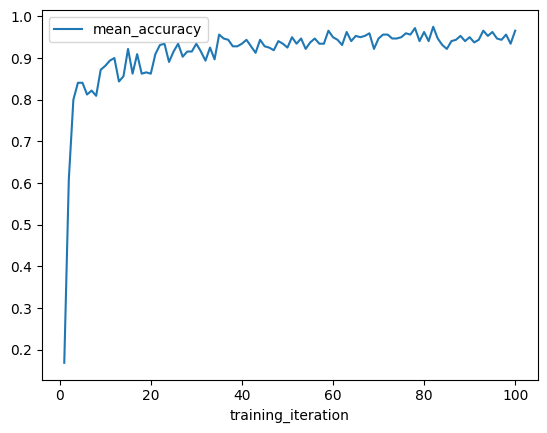
我们可以使用指标 DataFrame 快速可视化学习曲线。首先，让我们绘制最佳结果的平均准确率与训练迭代次数的关系图。

best_result.metrics_dataframe.plot("training_iteration", "mean_accuracy")

<AxesSubplot:xlabel='training_iteration'>

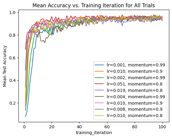
我们还可以迭代整个结果集，并创建所有试验的组合图，其中超参数作为标签。

ax = None
for result in result_grid:
    label = f"lr={result.config['lr']:.3f}, momentum={result.config['momentum']}"
    if ax is None:
        ax = result.metrics_dataframe.plot("training_iteration", "mean_accuracy", label=label)
    else:
        result.metrics_dataframe.plot("training_iteration", "mean_accuracy", ax=ax, label=label)
ax.set_title("Mean Accuracy vs. Training Iteration for All Trials")
ax.set_ylabel("Mean Test Accuracy")

Text(0, 0.5, 'Mean Test Accuracy')

访问检查点并加载以进行测试推理

前面我们看到 Result 包含与试验关联的最后一个检查点。让我们看看如何使用此检查点加载模型，以便对一些 MNIST 样本图像执行推理。

import torch

from ray.tune.examples.mnist_pytorch import ConvNet, get_data_loaders

model = ConvNet()

with best_result.checkpoint.as_directory() as checkpoint_dir:
    # The model state dict was saved under `model.pt` by the training function
    # imported from `ray.tune.examples.mnist_pytorch`
    model.load_state_dict(torch.load(os.path.join(checkpoint_dir, "model.pt")))

请参阅此处的训练循环定义，以了解我们最初是如何保存检查点的。

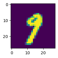
接下来，让我们用一个样本数据点测试我们的模型，并打印出预测的类别。

import matplotlib.pyplot as plt

_, test_loader = get_data_loaders()
test_img = next(iter(test_loader))[0][0]

predicted_class = torch.argmax(model(test_img)).item()
print("Predicted Class =", predicted_class)

# Need to reshape to (batch_size, channels, width, height)
test_img = test_img.numpy().reshape((1, 1, 28, 28))
plt.figure(figsize=(2, 2))
plt.imshow(test_img.reshape((28, 28)))

Predicted Class = 9

<matplotlib.image.AxesImage at 0x31ddd2fd0>

如果您想使用检查点模型进行大规模推理，请考虑使用 Ray Data！

总结

本指南中，我们探讨了一些可以使用 Tuner.fit 返回的 ResultGrid 输出执行的常见分析工作流程。其中包括：从实验目录加载结果、探索实验级和试验级结果、绘制记录的指标图，以及访问试验检查点进行推理。

请参阅Tune 的实验跟踪集成，了解更多您可以通过添加少量回调函数集成到 Tune 实验中的分析工具！