DLinear 模型使用离线批量推理进行验证

   

本教程演示了如何使用 DLinear 模型和 Ray Data 执行批量推理。该过程包括加载模型检查点、准备测试数据、批量运行推理以及评估性能。

请注意，此笔记本需要前一个“DLinear 时间序列模型的分布式训练”笔记本生成的预训练模型工件。

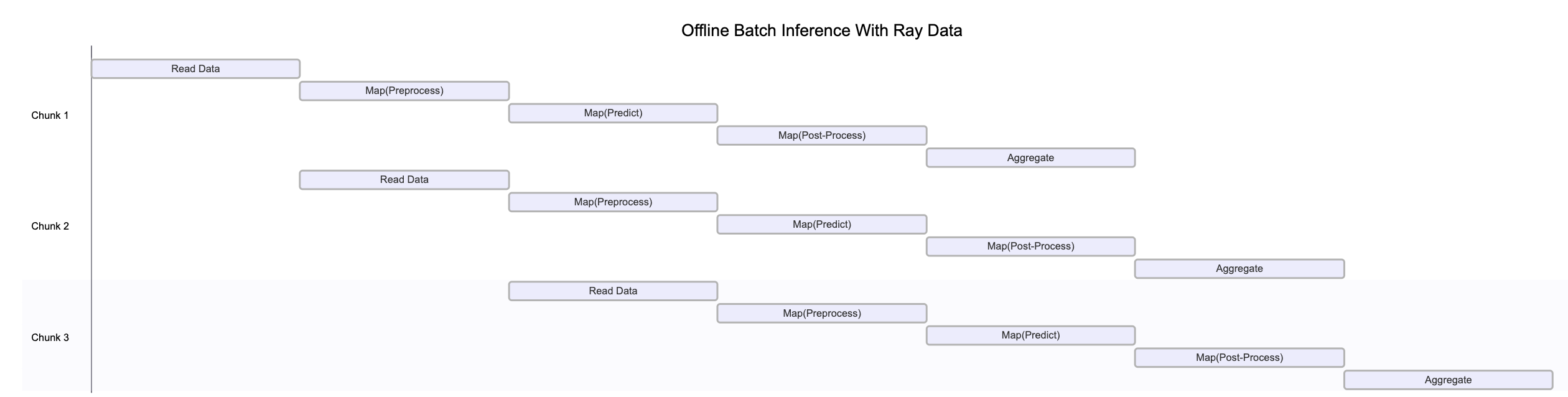
上图说明了数据块如何在管道的各个阶段并行处理。这种并行执行最大限度地提高了资源利用率和吞吐量。

请注意，此图表出于多种原因进行了简化

• 每个数据管道阶段只有一个工作进程

• 反压机制可能会限制上游运算符，以防止下游阶段过载

• 动态重分区通常发生在数据流经管道时，改变块的数量和大小

• 随着集群自动伸缩，可用资源会发生变化

• 系统故障可能会中断图中所示的整洁顺序流程

Ray Data 流式执行

❌ 传统的批量执行，非流式处理，例如没有流水线处理的 Spark 或 SageMaker Batch Transform

• 将整个数据集读入内存或持久的中间格式

• 然后才开始应用转换，例如 .map、.filter 等。

• 更高的内存压力和启动延迟

✅ Ray Data 的流式执行

• 在加载块后立即开始处理，无需等待整个数据集

• 减少内存占用，防止内存不足错误，并加快首次输出时间

• 通过减少空闲时间来提高资源利用率

• 能够以最小的延迟实现类似在线的推理管道

注意：Ray Data 以流式执行的批量处理方式运行，而不是像 Flink 或 Kafka Streams 这样的实时流处理引擎。这种方法对于迭代式机器学习工作负载、ETL 管道以及训练或推理前的预处理特别有用。与 Spark 和 SageMaker Batch Transform 等解决方案相比，Ray 通常能提供 2-17 倍的吞吐量提升。

# Enable importing from e2e_timeseries module.
import os
import sys

sys.path.insert(0, os.path.abspath(os.path.join(os.getcwd())))

首先设置环境和导入

import numpy as np
import ray
import torch

os.environ["RAY_TRAIN_V2_ENABLED"] = "1"

import e2e_timeseries
from e2e_timeseries.data_factory import data_provider
from e2e_timeseries.metrics import metric
from e2e_timeseries.model import DLinear

使用 e2e_timeseries 模块初始化 Ray 集群，以便新生成的 worker 可以导入它。

ray.init(runtime_env={"py_modules": [e2e_timeseries]})

接下来，设置 DLinear 模型配置和作业配置

# Load the best checkpoint path from the metadata file created in the training notebook.
best_checkpoint_metadata_fpath = os.path.join(
    "/mnt/cluster_storage/checkpoints", "best_checkpoint_path.txt"
)
with open(best_checkpoint_metadata_fpath, "r") as f:
    best_checkpoint_path = f.read().strip()

config = {
    "checkpoint_path": best_checkpoint_path,
    "num_data_workers": 1,
    "features": "S",
    "target": "OT",
    "smoke_test": False,
    "seq_len": 96,
    "label_len": 48,
    "pred_len": 96,
    "individual": False,
    "batch_size": 64,
    "num_predictor_replicas": 4,
}


def _process_config(config: dict) -> dict:
    """Helper function to process and update configuration."""
    # Configure encoder input size based on task type.
    if config["features"] == "M" or config["features"] == "MS":
        config["enc_in"] = 7  # ETTh1 has 7 features when multi-dimensional prediction is enabled
    else:
        config["enc_in"] = 1

    # Ensure paths are absolute.
    config["checkpoint_path"] = os.path.abspath(config["checkpoint_path"])

    config["num_gpus_per_worker"] = 1.0

    config["train_only"] = False  # Load test subset
    return config


# Set derived values.
config = _process_config(config)

数据摄取

首先，将测试数据集加载为 Ray Data Dataset。使用 .show(1) 来触发单行的执行，因为 Ray Data 是惰性求值的。

ray.init(ignore_reinit_error=True)

print("Loading test data...")
ds = data_provider(config, flag="test")
ds.show(1)

此单元定义了 Predictor 类。它从检查点加载训练好的 DLinear 模型，并处理输入批次以生成预测。call 方法对给定的 NumPy 数组批次执行推理。

Ray Data 的基于 actor 的处理允许仅加载一次模型权重并将其传输到 GPU，并在批次之间重复使用它们。

class Predictor:
    """Actor class for performing inference with the DLinear model."""

    def __init__(self, checkpoint_path: str, config: dict):
        self.config = config
        self.device = torch.device("cuda" if torch.cuda.is_available() else "cpu")

        # Load model from checkpoint.
        self.model = DLinear(config).float()
        checkpoint = torch.load(checkpoint_path, map_location=self.device)
        self.model.load_state_dict(checkpoint["model_state_dict"])
        self.model.to(self.device)
        self.model.eval()

    def __call__(self, batch: dict[str, np.ndarray]) -> dict:
        """Process a batch of data for inference (numpy batch format)."""
        # Convert input batch to tensor.
        batch_x = torch.from_numpy(batch["x"]).float().to(self.device)

        with torch.no_grad():
            outputs = self.model(batch_x)  # Shape (N, pred_len, features_out)

        # Determine feature dimension based on config.
        f_dim = -1 if self.config["features"] == "MS" else 0
        outputs = outputs[:, -self.config["pred_len"] :, f_dim:]
        outputs_np = outputs.cpu().numpy()

        # Extract the target part from the batch.
        batch_y = batch["y"]
        batch_y_target = batch_y[:, -self.config["pred_len"] :]

        return {"predictions": outputs_np, "targets": batch_y_target}

ds = ds.map_batches(
    Predictor,
    fn_constructor_kwargs={"checkpoint_path": config["checkpoint_path"], "config": config},
    batch_size=config["batch_size"],
    concurrency=config["num_predictor_replicas"],
    num_gpus=config["num_gpus_per_worker"],
    batch_format="numpy",
)

接下来，进行一些小的后处理，以获得所需维度的结果。

def postprocess_items(item: dict) -> dict:
    # Squeeze singleton dimensions for predictions and targets if necessary.
    if item["predictions"].shape[-1] == 1:
        item["predictions"] = item["predictions"].squeeze(-1)
    if item["targets"].shape[-1] == 1:
        item["targets"] = item["targets"].squeeze(-1)
    return item


ds = ds.map(postprocess_items)

最后，执行所有这些惰性步骤，并使用 take_all() 将它们具体化到内存中。

# Trigger the lazy execution of the entire Ray pipeline.
all_results = ds.take_all()

现在结果已在内存中，为训练好的 DLinear 模型计算一些验证指标。

# Concatenate predictions and targets from all batches.
all_predictions = np.concatenate([item["predictions"] for item in all_results], axis=0)
all_targets = np.concatenate([item["targets"] for item in all_results], axis=0)

# Compute evaluation metrics.
mae, mse, rmse, mape, mspe, rse = metric(all_predictions, all_targets)

print("\n--- Test Results ---")
print(f"MSE: {mse:.3f}")
print(f"MAE: {mae:.3f}")
print(f"RMSE: {rmse:.3f}")
print(f"MAPE: {mape:.3f}")
print(f"MSPE: {mspe:.3f}")
print(f"RSE: {rse:.3f}")

print("\nOffline inference finished!")